Quick start

Environnements

Maia is now distributed in elsA releases (since v5.2.01) ! Here is an extract of the embedded maia version number for the latest elsA releases (see elsA documentation for full list) :

elsA	5.2.03	5.3.01	5.3.02	5.3.03
maia	v1.2	v1.3.1	v1.4.1	v1.5

If you need more flexibility or if you want to try the latest features, maia releases are also deployed on Onera clusters. This is done through modulefiles, named following these conventions:

• 3 figures modules (eg maia/1.4.0) load the specified version;

• 2 figures modules (eg maia/1.4) load the latest available patchrelease (for example 1.4.2);

• maia/dev loads the latest build (which may be unstable, use it carefully);

• a suffix is used to indicate the compatible software socle, depending on the machine.

Spiro-EL8JunoSatorLD

module use --append /scratchm/sonics/usr/modules/
module load maia/dev-dsi-cfd6

For versions of maia up to 1.5, in addition to the DSI provided environments (socle-cfd/*), we also support the IntelMPI/GCC software chain used by former versions of Sonics. Those versions are suffixed by the "default" keyword and require the dependancies to be loaded manually, using this additional source command:

source /scratchm/sonics/dist/source.sh --env maia
module load maia/1.5-default

If you prefer to build your own version of Maia, see Installation section.

Supported meshes

Maia supports CGNS meshes from version 4.2, meaning that polyhedral connectivities (NGON_n, NFACE_n and MIXED nodes) must have the ElementStartOffset node.

Former meshes can be converted with the (sequential) maia_poly_old_to_new script included in the $PATH once the environment is loaded:

$> maia_poly_old_to_new mesh_file.hdf

The opposite maia_poly_new_to_old script can be used to put back meshes in old conventions, insuring compatibility with legacy tools.

Warning

CGNS databases should respect the SIDS. The most commonly observed non-compliant practices are:

• Empty DataArray_t (of size 0) under FlowSolution_t containers.

• 2D shaped (N1,N2) DataArray_t under BCData_t containers. These arrays should be flat (N1xN2,).

• Implicit BCDataSet_t location for structured meshes: if GridLocation_t and PointRange_t of a given BCDataSet_t differs from the parent BC_t node, theses nodes should be explicitly defined at BCDataSet_t level.

Several non-compliant practices can be detected with the cgnscheck utility. Do not hesitate to check your file if Maia is unable to read it.

Note also that ADF files are not supported; CGNS files should use the HDF binary format. ADF files can be converted to HDF thanks to cgnsconvert.

Highlights

Tip

Download sample files of this section: S_twoblocks.cgns, U_ATB_45.cgns

Daily user-friendly pre & post processing

Maia provides simple Python APIs to easily setup pre or post processing operations: for example, converting a structured tree into an unstructured (NGon) tree is as simple as

from   mpi4py.MPI import COMM_WORLD as comm
import maia

tree = maia.io.file_to_dist_tree('S_twoblocks.cgns', comm)
maia.algo.dist.convert_s_to_ngon(tree, comm)
maia.io.dist_tree_to_file(tree, 'U_twoblocks.cgns', comm)

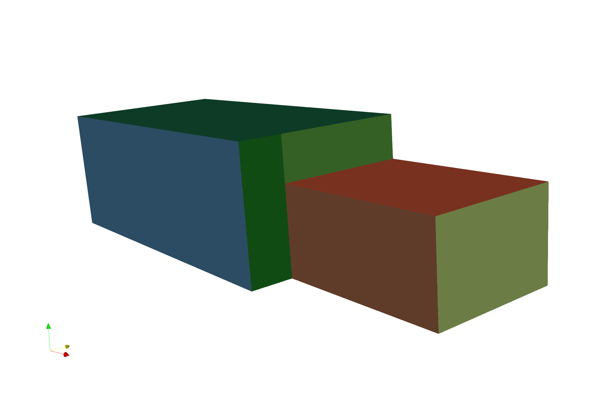
In addition of being parallel, the algorithms are as much as possible topologic, meaning that they do not rely on a geometric tolerance. This also allow us to preserve the boundary groups included in the input mesh (colored on the above picture).

Building efficient workflows

By chaining this elementary blocks, you can build a fully parallel advanced workflow running as a single job and minimizing file usage.

In the following example, we load an angular section of the ATB case, duplicate it to a 180° case, split it, and perform some slices and extractions.

from   mpi4py.MPI import COMM_WORLD as comm
import maia.pytree as PT
import maia

# Read the file. Tree is distributed
dist_tree = maia.io.file_to_dist_tree('U_ATB_45.cgns', comm)

# Duplicate the section to a 180° mesh
# and merge all the blocks into one
opposite_jns = [['Base/bump_45/ZoneGridConnectivity/matchA'],
                ['Base/bump_45/ZoneGridConnectivity/matchB']]
maia.algo.dist.duplicate_from_periodic_jns(dist_tree,
    ['Base/bump_45'], opposite_jns, 22, comm)
maia.algo.dist.merge_connected_zones(dist_tree, comm)

# Split the mesh to have a partitioned tree
part_tree = maia.factory.partition_dist_tree(dist_tree, comm)

# Now we can call some partitioned algorithms
maia.algo.part.compute_wall_distance(part_tree, comm, point_cloud='Vertex')
extract_tree = maia.algo.part.extract_part_from_bc_name(part_tree, "wall", comm)
slice_tree = maia.algo.part.plane_slice(part_tree, [0,0,1,0], comm,
      containers_name=['WallDistance'])

# Merge extractions in a same tree in order to save it
base = PT.get_child_from_label(slice_tree, 'CGNSBase_t')
PT.set_name(base, f'PlaneSlice')
PT.add_child(extract_tree, base)
maia.algo.pe_to_nface(dist_tree,comm)

extract_tree_dist = maia.factory.recover_dist_tree(extract_tree, comm)
maia.io.dist_tree_to_file(extract_tree_dist, 'ATB_extract.cgns', comm)

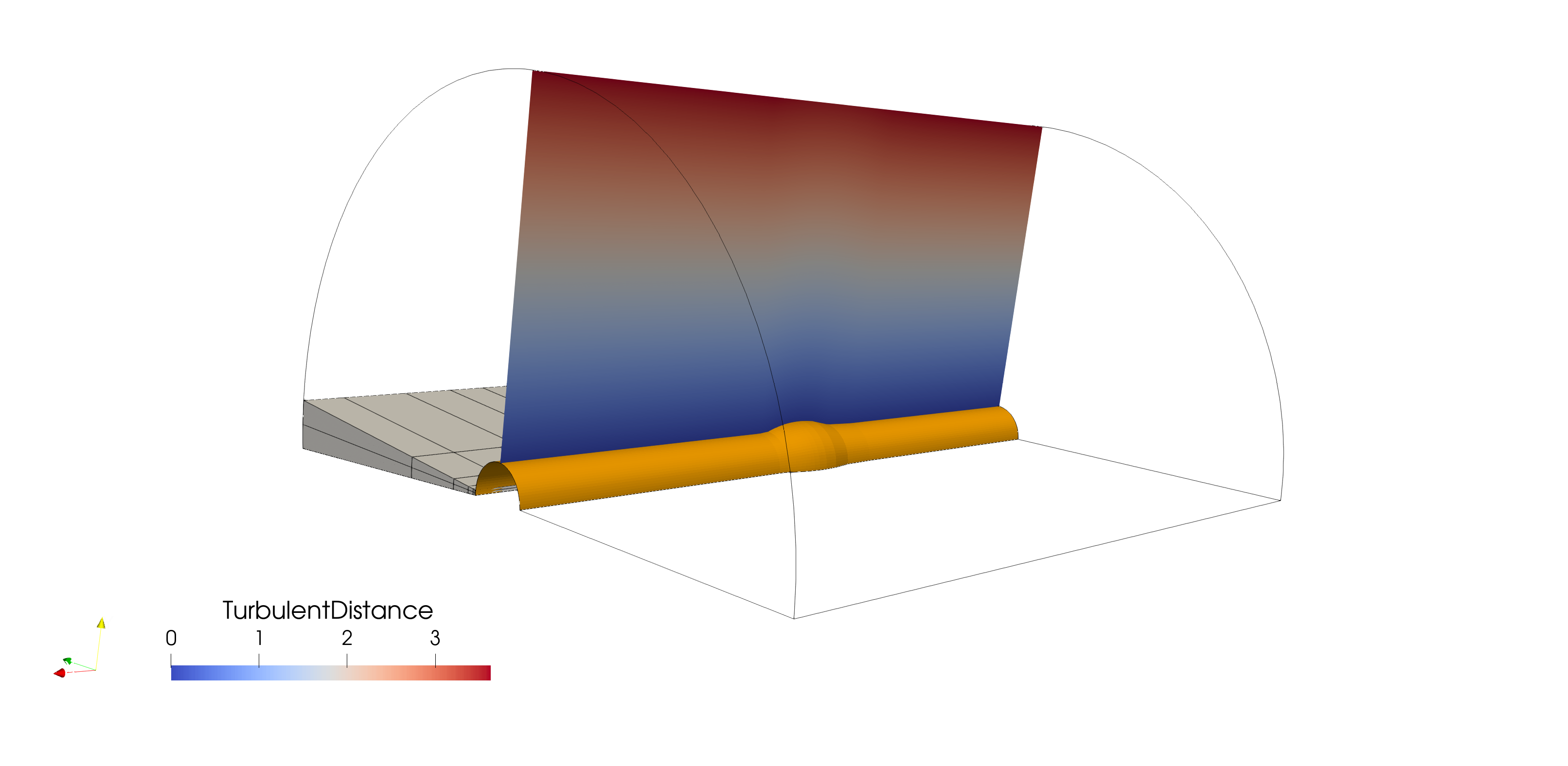
The above illustration represents the input mesh (gray volumic block) and the extracted surfacic tree (plane slice and extracted wall BC). Curved lines are the outline of the volumic mesh after duplication.

Compliant with the pyCGNS world

Finally, since Maia uses the standard CGNS/Python mapping, you can set up applications involving multiple python packages: here, we create and split a mesh with maia, but we then call Cassiopee functions to compute the gradient of a field on each partition.

from   mpi4py.MPI import COMM_WORLD as comm
import maia
import Transform.PyTree as CTransform
import Converter.PyTree as CConverter
import Post.PyTree      as CPost

dist_tree = maia.factory.generate_dist_block([101,6,6], 'TETRA_4', comm)
CTransform._scale(dist_tree, [5,1,1], X=(0,0,0))
part_tree = maia.factory.partition_dist_tree(dist_tree, comm)

CConverter._initVars(part_tree, '{Field}=sin({nodes:CoordinateX})')
part_tree = CPost.computeGrad(part_tree, 'Field')

maia.transfer.part_tree_to_dist_tree_all(dist_tree, part_tree, comm)
maia.io.dist_tree_to_file(dist_tree, 'out.cgns', comm)

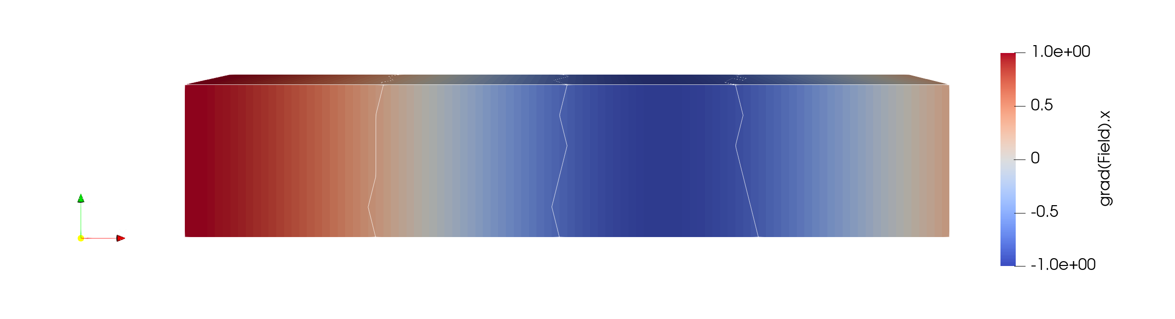
Be aware that other tools often expect to receive geometrically consistent data, which is why we send the partitioned tree to Cassiopee functions. The outline of this partitions (using 4 processes) are materialized by the white lines on the above figure.

Resources and Troubleshouting

The user manual describes most of the high level APIs provided by Maia. If you want to be comfortable with the underlying concepts of distributed and partitioned trees, have a look at the introduction section.

The user manual is illustrated with basic examples. Additional test cases can be found in the sources.

Issues can be reported on the gitlab board and help can also be asked on the dedicated Element room.